• WL100/45: Trois poèmes, UK*25 June 1969

It hardly seems possible that on this day 44 years ago I was about to conduct the UK premiere of Lutosławski’s Trois poèmes d’Henri Michaux (1963).  I shared the platform with the Nottingham University Chamber Choir and Orchestra and a fellow student conductor, Donald Goodhew.  Ever since I’d been introduced to this work in print and on LP in the autumn of 1968, I’d been totally captivated by it and its composer.  The rest, as they say, is history.  Less than a year later, I published a little article on the piece (possibly the first English-language journal article on Lutosławski’s music), focusing on its pitch organisation and our choral preparation.  Today I’ve posted this article – ‘A Deep Resonance’ (1970) – elsewhere on this site.

Graph of Lutosławski’s ‘Pensées’, not to temporal scale. © 2013 Adrian Thomas

One of the tools that I used to demonstrate how the choir (me) and the orchestra (Goodhew) interacted was by drawing up a graphic representation of the music as there was no combined score or ‘piano part’.  In order to do this, I had to carry out a detailed harmonic analysis.  The overall chart that I did in 1969 for the first movement, ‘Pensées’ (above), shows clearly the registral design of the music, the different forces (blue=wind, red=choir, green=pitched percussion), and symbolic graphic textures to indicate the changing musical textures.  While the harmonic dimension is regularly calibrated (one vertical mini-square on the graph represents a semitone), the temporal dimension is not to scale.  Middle C is the first horizontal band of mini-squares underlined by the next-to-lowest black line running left to right across the graph.  These five lines indicate the octave Cs.

One of the most intriguing sections runs from fig.35 to fig.84 (1’58”-3’19” in the recording above).  It is scored initially for seven woodwind instruments (3 flutes, 3 clarinets, 1 bassoon), a pared down echo of the ensemble of seven woodwinds that Lutosławski used in sections ACEG in the first movement of his previous work, Jeux vénitiens (this is far from being the only connection between the two pieces).  Characteristically, he changes the instrumentation almost by stealth over the course of the subsequent five iterations (the full complement of woodwind is 3 flutes, 2 oboes, 3 clarinets, 2 bassoons):

figs 35-45:  3.0.3.1
figs 46-53:  3.2.3.0
figs 54-59:  3.2.3.0
figs 61-64:  3.1.3.0
figs 66-72:  3.2.3.0
figs 74-84:  2.0.3.2

Each of the six short pp ‘clouds’ on the woodwind (blue) moves from one fixed point, usually a brief unison, to another in a different register – echoes here of the designs in the string sections BD(F)H in the first movement of Jeux vénitiens.  Interwoven are short contributions by the choral sopranos (red), with their own discrete pitch content.  It is a magical, quasi-stochastic texture.  These tail-less note heads seem completely free.

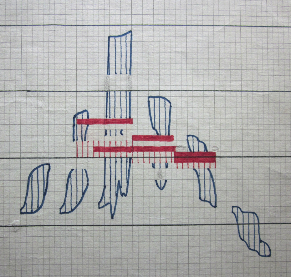
Graphic reduction of figs 35-84, Lutosławski’s ‘Pensées’ © 2013 Adrian Thomas

Yet that, of course, would be alien to Lutosławski’s way of thinking, let alone working.  He habitually worked up detailed maquettes of his ideas, and often in his music one senses its progress as a sequence of carefully matched sketches.  So it is here, not least in the range of different notational devices that he uses to create these clouds of sounds.  This second section from fig.35 to fig.84 is one of the most intriguing ‘sketches’.  I remember looking at it and realising that something was going on behind the apparent impressionism.  In the score, Lutosławski gives the advice: ‘Notes without tails indicate the shortest sounds possible.  The horizontal distances between the notes correspond approximately to the intervals of time (between the notes concerned)’.  This is a diversionary tactic.  In fact, these six textures are based on a single template, precisely worked out – it would seem – on graph paper.  At least, each of the one-second ‘bars’ can be matched up with the divisions of standard graph paper: 1 second = one large square of 1-inch graph paper subdivided into tenths (1″=1″, though obviously Lutosławski was not working with imperial measurements).

I worked out that there are two rhythmic strands at work, both of them mirror structures and both based on the principle of elasticity – the increase and decrease of rhythmic activity.  The distinction between the two strands may characterised this way: the flow of  ‘A’ is akin to accelerando-decelerando, while the flow of ‘B’ is regulated by addition-subtraction.  Both of these patterns relate to woodwind motifs in the first movement of Jeux vénitiens (sections ACEG).

‘A’ accelerando-decelerando

• the pattern is enunciated by fl.1 at fig.35: in intervals of 1/10th of a graph square, the acceleration moves from an initial gap of 12 down to 1 and back again, at which point it starts again: 12-8-4-2-1-1-2-4-8-12-8- etc..
• fl.2 begins with the second note of this accelerando, fl.3 with note 3, bassoon with note 4, each of them starting 1/10th of a graph square after its predecessor.   This way, the pattern is never discernible, not least because the pitch component is also different in each case.

‘B’ addition-subtraction

• the pattern is begun by cl.1, starting 1/10th of a graph square after the bassoon in pattern ‘A’.  It too has an accelerando-decelerando component, but is differentiated from ‘A’ by its additive-subtractive pattern: 1 note (a gap of 12/10ths), 2 notes (a gap of 9/10ths), 3 notes (a gap of 6/10ths), 4 notes (a gap of 5/10ths), 3 notes (a gap of 8/10ths), 2 notes (a gap of 11/10ths), 1 note (a gap of 12/10ths), etc..  In sum: 1-(12)-2-(9)-3-(6)-4-(5)-3-(8)-2(11)-1 (12)-2- etc..
• as with ‘A’, subsequent entries start 1/10th of a graph square after the preceding one: cl.1 (1 note) is followed by cl.2 starting with the group of 2 notes, cl.3 starting with the group of 3 notes.

All together now

Here is my marked-up score from 1969 of the first ‘cloud’ (figs 35-43; figs 44-45 are on the next system), with each note of the ‘A’ pattern marked as the 1st, 2nd, etc. up to ‘6’.  You can also see the cut-off points for subsequent ‘clouds’.

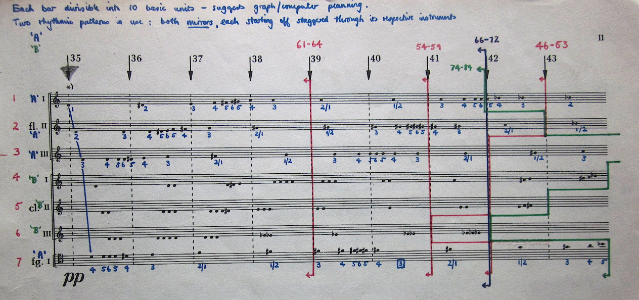
Figs 35-43, Lutosławski’s ‘Pensées’ © 1965 PWM; annotations © 2013 Adrian Thomas

The first of the six ‘clouds’ provides the fullest statement (lengthwise) of the combined rhythmic templates of ‘A’ and ‘B’, though a fourth contribution to ‘B’, starting with the group of 4 notes, is introduced in the second ‘cloud’ (ob.2).  All the other five ‘clouds’ may be understood as excerpts from the first one, with Lutosławski ringing the changes in the sequence of instrumental entries:

figs 35-45:  ten ‘bars’ (incomplete)
figs 46-53:  eight ‘bars’ = figs 35-43 (incomplete)
figs 54-59:  six ‘bars’ = figs 35-40
figs 61-64:  four ‘bars’ = figs 35-38
figs 66-72:  seven ‘bars’ = figs 35-42
figs 74-84:  ten ‘bars’ = figs 35-44 (incomplete)

As the indication ‘incomplete’ above reveals, Lutosławski does not follow this canonic layering slavishly.  The sixth ‘cloud’ not only omits some of the final notes but also inserts the ones missing from the first ‘cloud’ (compare figs 81-84 with 42-45).  Elsewhere, there are quite a few places where Lutosławski has missed out notes (or occasionally added them), for no apparent compositional reason.  Might one dare to suggest that creative hurry was the cause? The list includes 46 (cl.1), 51 (ob.1); 54 (cl.3), 55 (ob.1), 56-57 (fl.2), 59 (fl.1-2, ob.2, cl.3); 71 (ob.1); 74 (fl.2), 81 (fl.1, cl.3), 82 (fl.1-2, cl.2-3), 83 (fl.1-2, cl.1-3, fg.1-2).

Lutosławski did not use this notation again.  But many of the ideas he explored here and elsewhere in ‘Pensées’ resurface in related forms in subsequent pieces, not least the principle that a texture that sounds uncomplicated should in fact have quite a rigorous underpinning, however disguised that may be.